ivd: an R package for individual variance detection
A holistic view of academic performance: Beyond Averages with MELSM and Spike-and-Slab
Marwin Carmo 1
mmcarmo@ucdavis.edu
Donald R. Williams 1
drwwilliams@ucdavis.edu
Philippe Rast 1
prast@ucdavis.edu
1 University of California, Daviss
Introduction
To get a more complete picture of academic achievement of a student or a school, it’s important to look at both average performance and variability within a cluster. We adapted the mixed-effects location scale model (MELSM) using the Spike and Slab regularization technique to shrink the scale random effects to their fixed effect. This allows us to identify clusters with unusually (in)consistent academic achievement.
Model formulation
The random effects from the scale and location can be modeled as, \(\textbf{u}\sim\mathcal{N}(\textbf{0}, \boldsymbol{\Sigma})\). The covariance matrix of the random effects can be decomposed into \(\boldsymbol\Sigma = \boldsymbol{\tau}\boldsymbol{\Omega\tau}'\) to specify independent priors for each element of \(\boldsymbol{\tau}\) (random-effects standard deviations) and \(\boldsymbol{\Omega}\) (correlation matrix among all random effects).
\(\boldsymbol\Omega\) can be factorized via the Cholesky \(\textbf{L}\) of \(\boldsymbol\Omega = \textbf{L}'\textbf{L}\). Then, \(\textbf{u}\) can be recovered multiplying \(\textbf{L}\) by the random effect standard deviations, \(\boldsymbol{\tau}\), and scaling it with a standard normally distributed \(\boldsymbol{z}\).
An indicator variable (\(\delta\)) is included in the prior for the scale random effect to allow switching between the spike and slab throughout the MCMC sampling process. For each school \(j\), we obtain a probabilistic measure on whether the scale random effect is to be included or not:
\[\textbf{u}_j = \boldsymbol{\tau}\textbf{L}\color{red}{\boldsymbol{\delta}}_j\textbf{z}_j\] For a random intercept only model,
\[\begin{equation} \label{eq:mm_delta} \alpha_{0j} = \begin{cases} \eta_{0}, & \text{if }\delta_j = 0 , \\ \eta_{0} + u_{0j}, & \text{if }\delta_j = 1 \end{cases}. \end{equation}\]
The posterior inclusion probabilities (PIP) can then be computed as
\[\begin{align} Pr(\alpha_{0j} = \eta_{0} | \textbf{Y}) = 1 - \frac{1}{S} \sum_{s = 1}^S \delta_{js}, \end{align}\]
where \(S = \{1,...,s\}\) denotes the posterior samples and \(\eta_{0}\) is the average within-person variability.
The methods have been implemented in the R package ivd:
devtools::install_github("consistentlybetter/ivd")Illustrative example
The data comes from The Basic Education Evaluation System (Saeb) conducted by Brazil’s National Institute for Educational Studies and Research (Inep) in 2021. It is also available as the saeb dataset in the ivd package. The outcome variable is math_proficiency at the end of grade 12. Location and scale are modeled as a function of student and school SES.
out <- ivd(location_formula = math_proficiency ~ student_ses * school_ses + (1|school_id),
           scale_formula =  ~ student_ses * school_ses + (1|school_id),
           data = saeb,
           niter = 5000, nburnin = 5000, WAIC = TRUE, workers = 4)
Results
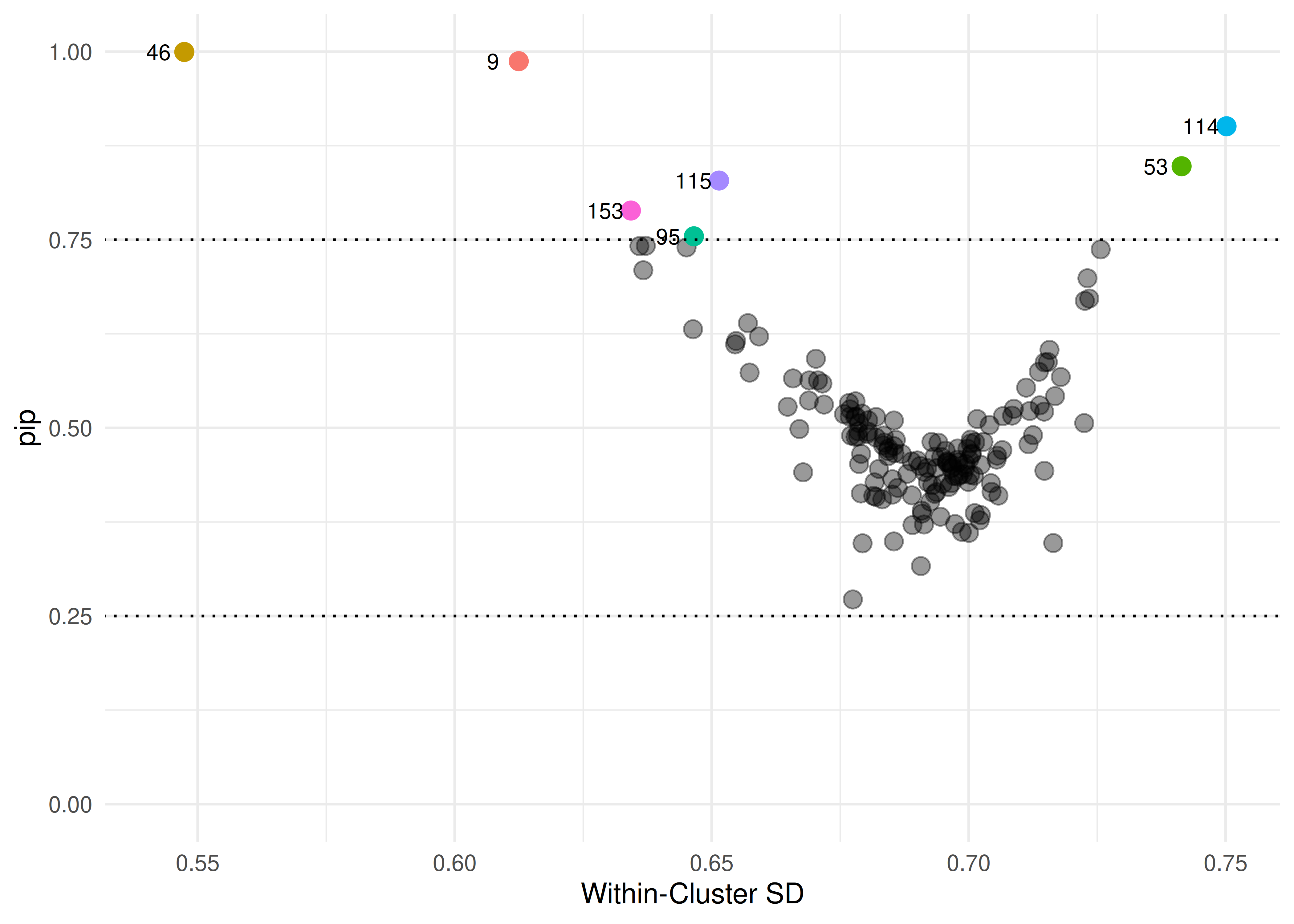
Figure 1: Funnel plot of posterior inclusion probabilities and school’s standard deviations. Higher PIP values express more evidence for the random effect of a given school to be included in the model.
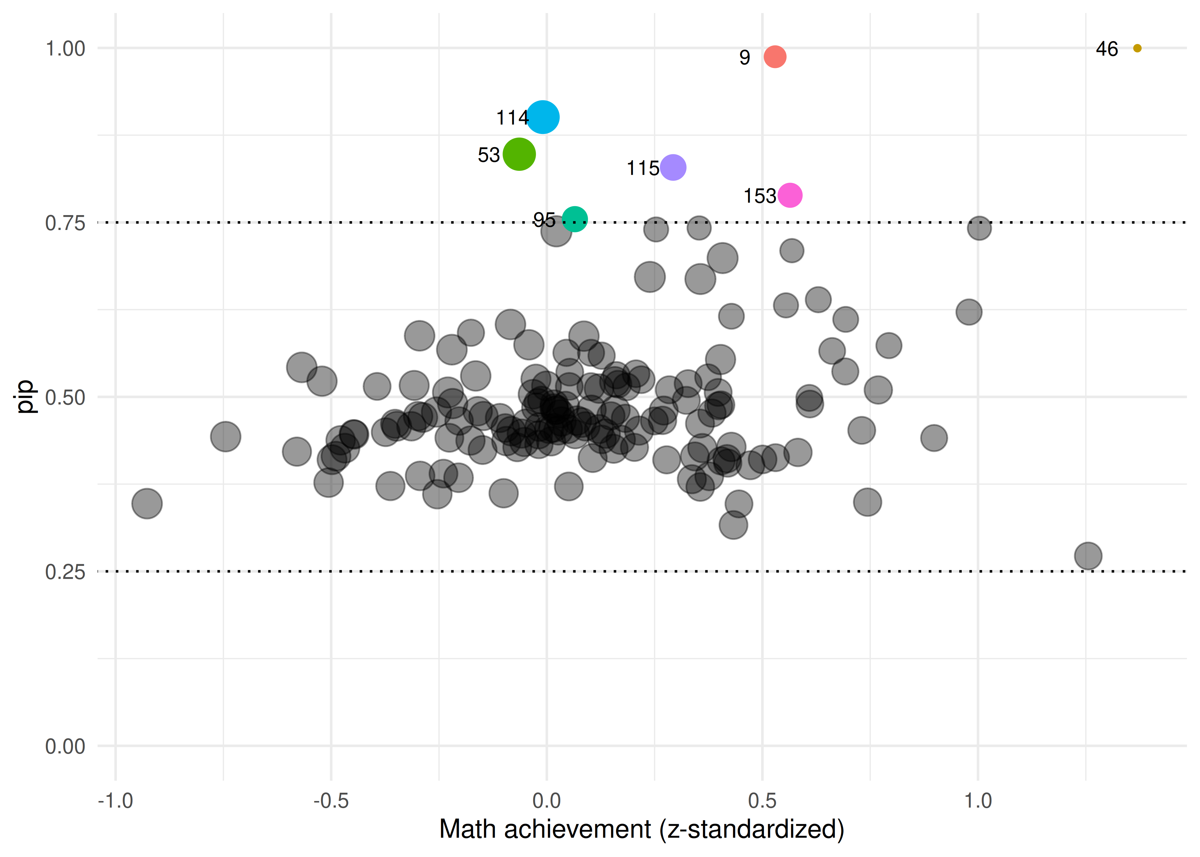
Figure 2: Posterior inclusion probabilities plotted against school’s average math achievement in standardized units. Point size represents within-school standard deviation.
Discussion
Individual variance detection analysis suggests that some schools have students consistently performing above the average, while others have an average mean score but with greater-than-average variability. Inconsistent performance may reflect unaccounted factors influencing learning.
The IVD method could also be used to assess academic performance throughout the year and uncover information relevant to providing more specific school or student support.
The
ivdpackage is an accessible tool for applying the spike-and-slab prior to the scale random effects in mixed-effects models for individual differences research. It aids researchers in identifying units that deviate from the average variance effect.
References
Rodriguez, J. E., Williams, D. R., & Rast, P. (2024). Who is and is not" average’"? Random effects selection with spike-and-slab priors. Psychological Methods. https://doi.org/10.1037/met0000535
Williams, D. R., Martin, S. R., & Rast, P. (2022). Putting the individual into reliability: Bayesian testing of homogeneous within-person variance in hierarchical models. Behavior Research Methods, 54(3), 1272–1290. https://doi.org/10.3758/s13428-021-01646-x
