Using the same dataset for variable selection, parameter estimation, and inference invalidates classical guarantees. I use simulations to show how post-selection sampling distributions become distorted, and identify the conditions—noise, sample size, and predictor correlation—that make things worse.
Much of the current research questions on behavioral and social sciences are investigated using statistical models (Flora, 2017). Models are simplified translations of a reality to mathematical expressions; its’ aim is to express how data were generated. Regression-based models are vastly employed in empirical research and often used to estimate causal effects (Berk, 2010). However, to perform causal modeling, researchers must specify a “correct” model (i.e., an accurate model of the data generating process) prior to data collection and use the obtained data only to estimate regression coefficients (see Berk (2010) for further discussion). In practice, researchers usually only have a vague idea of the right model to answer their research questions, or even if such model can be estimated. Often, what is framed as statistical inference or causal modeling is in fact a descriptive analysis; what Berk (2010) name as Level I Regression Analysis.
To determine which variables should be included in the model, a common solution is to resort to variable selection algorithms. The drawback is that whenever data-driven variable selection procedures are employed, classical inference guarantees are invalidated due to the model itself becoming stochastic(Berk et al., 2013). It means that if the model selection method evaluates the stochastic component of the data, the model is also considered stochastic.
Why is it a problem?
Variable selection procedures aren’t in themselves problematic. Nevertheless, when the correct model is unknown prior to data analysis, and the same dataset is used for I) variable selection, II) parameter estimation, and III) statistical inferences, the estimated results can be highly biased. This is because we add a new source of uncertainty when performing model selection. These procedures discards parameter estimates from the model, and, as we shall see, the sampling distribution of the remaining regression parameters estimates gets distorted. In addition, the selected model isn’t the same across samples, so there is another source of uncertainty to the estimates. (Berk et al., 2010).
Consider a well defined population with its unknown regression parameter values. We draw a random sample and apply a model selection procedure. The “best” model found by the variable selection is sample specific and isn’t guarantee to be the correct model (if we assume that such model in fact exists). Suppose we repeat the process of drawing a random sample and performing model selection 10,000 times. In this example there are six possible candidates, and only one correct model. We can simulate the expected frequency in which each of these models is chosen given a probability of 1/3 for the correct model and 1/9 otherwise. As shown in the following table, even if the correct model (in this case, \(\hat{M}_2\)) is three times more likely to be selected than the competing models, it is expected to be chosen more frequently but not at the majority of the time. Therefore, the expected selected model is an incorrect one.
To understand why the regression parameters estimates might be biased, recall that in a multiple regression we estimate partial regression coefficients: in a regression equation, the weight of independent variables are estimated in relation to the other independent variables in the model (Cohen & Cohen, 1983). For a dependent variable, \(Y\), predicted by variables \(X_1\) and \(X_2\), \(B_{Y1 \cdot 2}\) is the partial regression coefficient for \(Y\) on \(X_1\) holding \(X_2\) constant, and \(B_{Y2 \cdot 1}\) is the partial regression coefficient for \(Y\) on \(X_2\) holding \(X_1\) constant. This regression equation is written as:
where \(B_{Y0 \cdot 12}\) is the model intercept when \(X_1\) and \(X_2\) are held constant and \(\varepsilon\) is the error term.
The regression coefficient for \(X_i\), for \(i = \{1, 2\}\), is model dependent. To see why, let’s take a look at the equations for the regression coefficients for \(X_1\) (\(B_{Y1 \cdot 2}\)) and \(X_2\) (\(B_{Y2 \cdot 1}\))
Here \(\rho\) stands for the populational correlation coefficient and \(\sigma\) for the populational standard deviation. Unless we have uncorrelated predictors (i.e. \(\rho_{12}\) = 0), the value for any of the regression coefficients is determined by which other predictors are in the model. If either one is excluded from the model, a different regression coefficient will be estimated: excluding \(X_2\), for example, would zero all the correlations involving this predictor, leaving,
Berk et al. (2010) warns that the sampling distribution of the estimated regression parameters is distorted because estimates made from incorrect models will also be included, resulting in a mixture of distributions. Therefore, the model selection process must be taken into account in the regression estimation whenever it is applied.
Illustration
We can illustrate the discussion above expanding an analytic example given by Berk et al. (2010) with simulations. Consider a model for a response variable \(y\) with two potential regressors, \(x\) and \(z\). Say we are interested in the relationship between \(y\) and \(x\) while holding \(z\) constant, that is, \(\hat{\beta}_{yx\cdot z}\). Framing this as a linear regression model we have
Now, suppose that we’re in a scenario where \(\rho_{xz}\) = 0.5, both \(\beta_1\) and \(\beta_2\) are set to 1 and \(\varepsilon \sim N(0, 10)\). We’ll use a sample size of 250 subjects, and 1,000 random samples will be drawn from this population. We’ll calculate coverage and bias for each regressor. Coverage informs the frequency in which the true coefficient value is captured by the 95% confidence interval (CI) of the estimate. The bias of the estimations is calculated as \(\frac{1}{R}\sum(\hat{\theta_r}-\theta)\), where \(R\) is the number of repetitions, \(\theta\) represents a population parameter, and \(\hat{\theta}_r\) a sample estimate in each simulation.
Code
p <-2# number of predictorsSigma <-matrix(.5, p, p) # correlation matrixdiag(Sigma) <-1n =250# sample sizeb0 <-10# intercept (can be set to any value)betas <-rep(1, 2)reps =1000coefs <- cover <-matrix(0, nrow = reps, ncol =2) # defining the matrices to store simulation resultsfor (i inseq(reps)) {# X is a matrix of regression coefficients X <- MASS::mvrnorm(n = n, rep(0, 2) , Sigma)# with the values randomly drawn in X, we'll estimate values for y y <-as.numeric(cbind(1, X) %*%c(b0, betas) +rnorm(n, 0, sqrt(10))) Xy <-as.data.frame( cbind(X, y))colnames(Xy) <-c(c("x", "z"), "y")# fit a linear model with x and z to predict y fit <-lm(y ~ ., data = Xy) coefs[i, ] <-coef(fit)[-1] # save the regression coefficients cis <-confint(fit)[-1,] # save the 95% CIs# if the true value is capture by the CI, sum 1, 0 otherwise cover[i,] <-ifelse(cis[,1] <1& cis[,2] >1, 1, 0)}colnames(coefs) <-c("x", "z")coefs <-as.data.frame(coefs)tibble::tibble(Predictor =c("x", "z"),Coverage =colMeans(cover),Bias =colMeans(coefs - betas)) |> knitr::kable()
Predictor
Coverage
Bias
x
0.942
-0.0072621
z
0.947
-0.0015634
Code
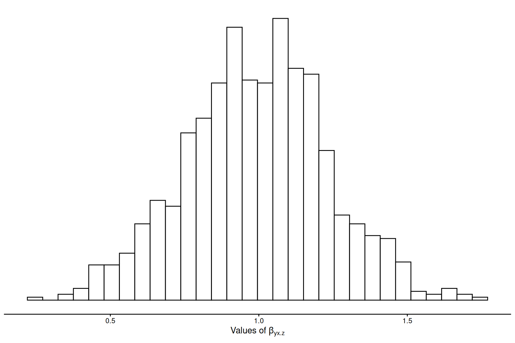
ggplot(data = coefs, aes(x = x)) +geom_histogram(color ="black", fill ="white", bins =30) +theme_classic() +theme(axis.title.y=element_blank(),axis.text.y=element_blank(),axis.ticks.y=element_blank(),axis.line.y =element_blank()) +xlab( expression(paste("Values of ", beta[yx.z])))
Sampling distributions of the regression coefficient for regressor \(x\) in the full model.
In this first scenario \(\beta_{yx\cdot z}\) is estimated assuming \(x\) and \(z\) are always included in the model.
What would happen if by model selection we arrive at a model where \(z\) is excluded? As indicated in Equation 2, if \(z\) is excluded, any correlation where \(z\) is involved is equivalent to zero, and we’re left with,
Note that \(\beta_{yx}\) is not the same as \(\beta_{yx\cdot z}\). If we do not have a model specified prior to data collection and analysis, it is not clear which definition of regression parameter for \(x\) we’re trying to estimate, if \(\beta_{yx\cdot z}\), as exemplified on Equation 1, or if \(\beta_{yx}\) from Equation 3. Therefore, the definition of \(\hat{\beta}_1\) depends on the model in which it is placed.
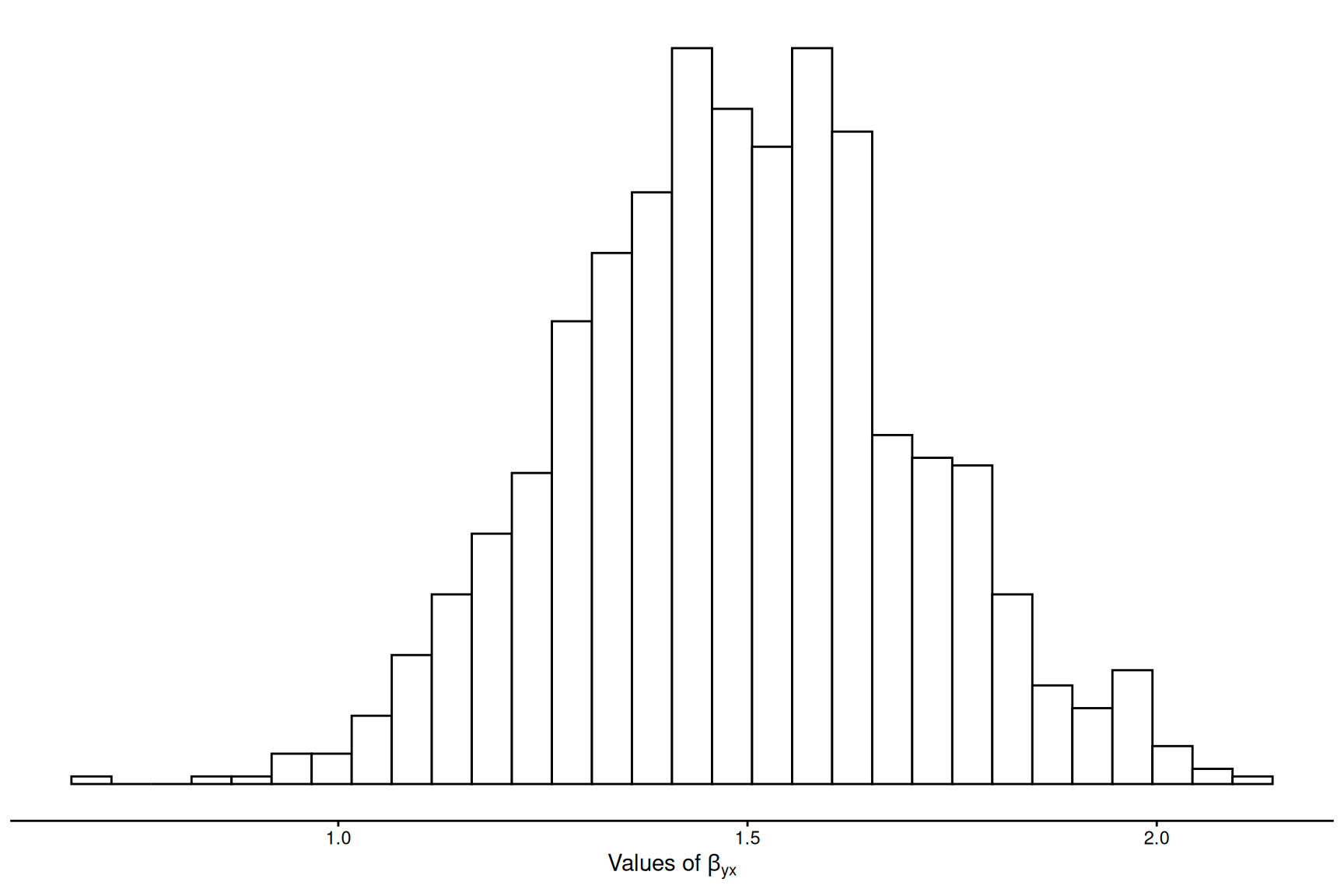
ggplot(data = coefs, aes(x = x)) +geom_histogram(color ="black", fill ="white", bins =30) +theme_classic() +theme(axis.title.y=element_blank(),axis.text.y=element_blank(),axis.ticks.y=element_blank(),axis.line.y =element_blank())+xlab( expression(paste("Values of ", beta[yx])))
Sampling distributions of the regression coefficient for regressor X in a reduced model where Z is excluded.
Notice how far off the model estimates the coefficient for \(x\) when we fit our model as y ~ x. Under these conditions, we should expect a coverage of the true coefficient value of \(x\) of 0.359 and a bias of 0.283. Under the correct model, bias is negligible and coverage follows the Type I error rate of 5% that we’ve set for this exercise.
This simple example help us understand why estimating model parameters in the same single random sample used to find an appropriate model isn’t a good idea (at least not without taking this process into account prior to making inferences). Discarding \(z\) from our model has distorted the sampling distribution of \(x\). Thus, as Berk et al. (2010) puts it: “when a single model is not specified before the analysis begins, it is not clear what population parameter is the subject of study. And without this clarity, the reasoning behind statistical inference becomes obscure”.
Other issues
We already know that if two predictors are moderately correlated and one is dropped from the model, our estimation will be biased. But what else should we consider? If we are selecting the variable every time, then there is not an issue. In the following sections we’ll consider what can make things go “bad”. Before that, please consider the equation for the standard error of the regression coefficient, estimated in the example model selection,
We have that \(\hat{\sigma_{\varepsilon}}\) is an estimate of the residual standard deviation, \(s_x\) is the sample standard deviation of \(x\), \(r^2_{xy}\) is the square of the sample correlation between \(x\) and \(z\), and \(n\) is the sample size. If the standard error for a regression coefficient is large, it means that its distribution will be more dispersed. So, from this equation, we identify as crucial parameters for a wider sampling distribution: larger residual variance, less variance in \(x\), smaller sample size, and, stronger correlation between regressors and the response variable.
We’ll use simulated data to aid our understanding. I have build a ShinyApp for that end. Its purpose is to illustrate the problems that arise when model selection, parameters estimation and statistical inferences are undertaken with the same data set. Although I will be working with code in this post, most of it can also be reproduced with this app.
For convenience purposes, I’ll use the stepwise approach for model selection with AIC as model selection criterion. Some penalties are harsher than others, but the concerns raised here are irrespective of the chosen model selection method (Berk et al., 2010). In the app, I also provide the option to choose BIC or Mallow’s Cp as selection method. In addition to bias and coverage, we’ll also estimate the average Mean Squared Error (MSE), calculated as \(\frac{1}{R}\sum[(\hat{\theta_r}-\theta)^2]\).
Noise
To express variability we can use a signal-to-noise ratio (SNR), defined here as:
where, \(\textbf{b}\) is a (p + 1) vector of regression coefficients, \(\Sigma\) is the covariance matrix of predictors and \(\sigma^2\) is the error term variance. Note that “model selection bias also occurs when an explanatory variable has a weak relationship with the response variable. The relationship is real, but small. Therefore, it is rarely selected as significant” (Lukacs et al., 2009, p. 118). We can experiment with a range of values for the \(SNR\) to see how it affects the estimates. We’ll use most values set in our first simulation exercise and \(SNR\) values ranging from 0.1 to 2. One thousand (1,000) simulations will be run for each of those values.
sim_snr <- purrr::pmap_dfr(list(reps =1000, p =2, n =250, SNR =c(.01, .1, .5, 1, 2), 1, corr =0.5), sim_bias)sim_snr |> knitr::kable()
SNR
N
Predictor
Estimate
Coverage
Bias
MSE
0.01
250
x1
2.2073663
0.333
1.2073663
2.9517905
0.01
250
x2
2.2889150
0.247
1.2889150
3.1180601
0.10
250
x1
1.1212326
0.820
0.1212326
0.1232157
0.10
250
x2
1.1265160
0.822
0.1265160
0.1481413
0.50
250
x1
0.9992872
0.957
-0.0007128
0.0323090
0.50
250
x2
1.0010014
0.955
0.0010014
0.0310951
1.00
250
x1
0.9975253
0.944
-0.0024747
0.0164856
1.00
250
x2
1.0007779
0.948
0.0007779
0.0164894
2.00
250
x1
1.0039598
0.937
0.0039598
0.0080606
2.00
250
x2
1.0012029
0.931
0.0012029
0.0088542
As expected, with greater amount of noise in relation to signal, the selected model includes the true coefficient at smaller frequencies. Because model selection interferes with the true model composition, coefficient estimates deviate from its true value. In this particular setting, with \(SNR\)\(\ge\) 0.5, coverage frequency approximates 95% and the estimates get closer to their true value. Measures of bias and MSE are also useful to display how our uncertainty gets smaller with less variability in the data.
Sample size
Once we know Equation 4 it is not difficult to suppose that larger samples produce smaller standard errors for the regression coefficients. We can confirm that using our sim_bias function again, but this time varying sample sizes.
Code
sim_ss <- purrr::pmap_dfr(list(reps =1000, p =2, n =c(10, 50, 100, 200, 500), SNR =0.5, b =1, corr =0.5), sim_bias)sim_ss|> knitr::kable()
SNR
N
Predictor
Estimate
Coverage
Bias
MSE
0.5
10
x1
1.7504550
0.432
0.7504550
1.7268897
0.5
10
x2
1.7334193
0.424
0.7334193
1.8854553
0.5
50
x1
1.1480525
0.806
0.1480525
0.1527022
0.5
50
x2
1.1325242
0.795
0.1325242
0.1462662
0.5
100
x1
1.0103067
0.949
0.0103067
0.0745612
0.5
100
x2
1.0064552
0.926
0.0064552
0.0784238
0.5
200
x1
0.9922657
0.949
-0.0077343
0.0417126
0.5
200
x2
0.9950722
0.940
-0.0049278
0.0430476
0.5
500
x1
1.0008457
0.951
0.0008457
0.0157077
0.5
500
x2
0.9983265
0.951
-0.0016735
0.0159465
Candidate predictors
OK, so far we’ve seen that with 2 predictors, each with true coefficient values of 1 and a correlation of 0.5, we get more precise estimates when \(SNR \ge\) 0.5 and \(n \ge\) 100. The number of candidate predictor variables and its covariance matrix are two important aspects not addressed yet. To demonstrate their influence we can run simulations with varying values for each, where each case will have a different combination of number of predictors and correlation between them.
For simplicity, all the off-diagonal elements the correlation matrix of predictors will be equal, meaning the that every predictor in the full model is correlated with the others by the same degree. We’ll need to do a slight modification on our previous function so we can then apply a new function for each combination and build a dataframe summarizing our results.
To keep the computing load at reasonable levels, we’ll limit the length of vectors of \(p\) and \(\rho\) to 10 values each. Our grid for \(\rho\) ranges from 0.1 to 0.9 and we’ll increase \(p\) from 2 to 10. We’ll set \(SNR\) = 0.5, \(n\) = 100 and set all true coefficient values to 1. Again, we’re using AIC to select the best model, and performing 1,000 simulation replicates.
Code
future::plan(future::multisession)sims <- furrr::future_map(seq(2, 10),~furrr::future_pmap(list(reps =1000, p = .x, n =100, SNR =0.5, 1,corr =seq(0.1, 0.9, by =0.1)), sim_bias_multi),seed=TRUE)simdf <- sims |> purrr::flatten() |> purrr::map(sim_summary) |> dplyr::bind_rows()
Code
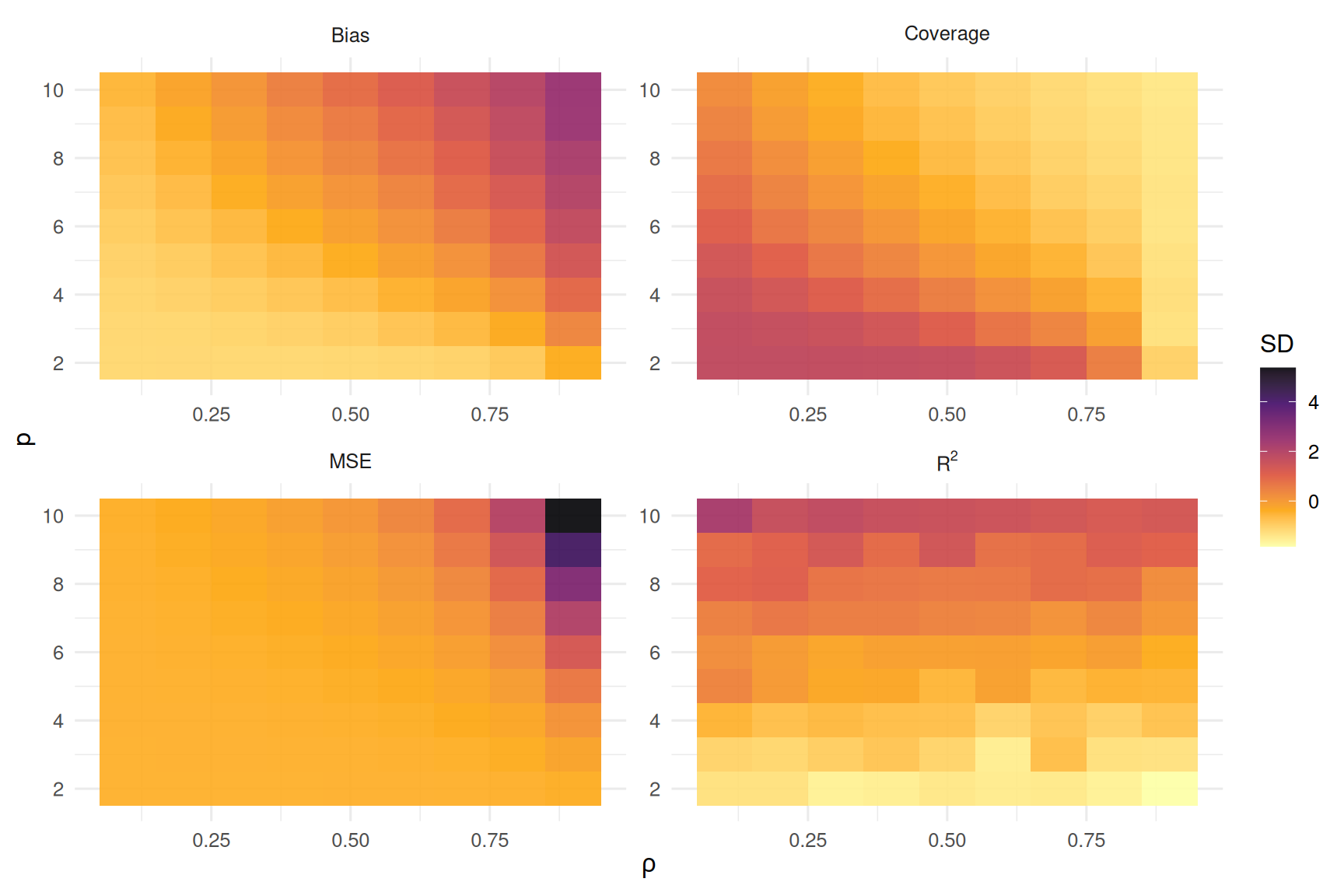
#| fig-cap: "Standardized measures of Bias, Coverage, Mean Square Error (MSE) and R2, across each simulation of pairs of number of predictors and correlation values"#| message: false#| dpi: 300simdfplot <- simdf |> dplyr::group_by(cor, npred) |> dplyr::summarise(coverage =mean(coverage),estimate =mean(estimate),bias =mean(bias),mse =mean(mse),rsq =mean(rsq)) |> dplyr::ungroup()simdfplot |> dplyr::mutate(dplyr::across(c("coverage", "bias", "mse", "rsq"), scale)) |> tidyr::pivot_longer(cols =c(coverage, bias, mse, rsq), names_to ="measure", values_to ='value') |> dplyr::mutate(measure = dplyr::recode(measure, "coverage"="Coverage", "bias"="Bias", "mse"="MSE", "rsq"="R^2")) |>ggplot() +aes(x = cor, y = npred, fill = value) +geom_tile() +scale_fill_viridis_c(direction =-1, option ="inferno", alpha = .9) +scale_y_continuous(breaks =c(2, 4, 6, 8, 10)) +labs(x = latex2exp::TeX("$\\rho$"), y ="p", fill ="SD") +theme_minimal(12) +facet_wrap(~measure, scales ="free",labeller = label_parsed)
To keep all four plots in the same scale, I have standardized the horizontal axis values. In this heat map, darker colors represent larger values (greater standard deviation). The pattern for Bias and MSE is similar: performing model selection with a great number of highly correlated predictors is likely to produced highly biased estimates. As expected, Coverage follows an inverted pattern from Bias and MSE: highly biased estimates fall out of the 95% CI coverage.
These plots make clear that our best case scenario is to have few, weakly correlated predictors. Of course, this is a setting rarely seen in empirical research – whats the point of going through model selection if you have only a handful of variables? What should really get our attention here is that bias in estimates is likely to get bigger if model selection is naively performed with little prior information about the data generating system to filter out candidate models. We have seen that sample size, SNR, number of predictors, and correlation between parameters with themselves and with the response variable, are characteristics of the model that each in their own way contributes to producing biased estimates. I encourage you to use this companion shinyapp to play with different scenarios to practice what we’ve been discussing so far.
Visualizing distributions
We’ve discussed earlier how dropping a predictor from the model can distort the coefficient sampling distribution of the remaining ones when they’re not orthogonal. However, even when the preferred (or “correct”) model is selected, there is no guarantee about obtaining sound regression coefficient estimates. In this final example, we’ll show that if by chance the “correct” model is achieved by model selection, the sampling distributions of the resulting regression coefficients might be different whether we condition on arriving at the correct model or on the correct model being known in advance.
Consider this example from Berk et al. (2010). As with the other examples, we’ll implement forward stepwise regression using the AIC as a fit criterion. The full regression model takes the form of
where \(\beta_0\) = 3.0, \(\beta_1\) = 0.0, \(\beta_2\) = 1.0, and \(\beta_3\) = 2.0. The variances and covariance are set as: \(\sigma^2_\varepsilon\) = 10.0, \(\sigma^2_w\) = 5.0, \(\sigma^2_x\) = 6.0, \(\sigma^2_z\) = 7.0, \(\sigma_{w,x}\) = 4.0, \(\sigma_{w,z}\) = 5.0, and \(\sigma_{x,z}\) = 5.0. The sample size is 200.
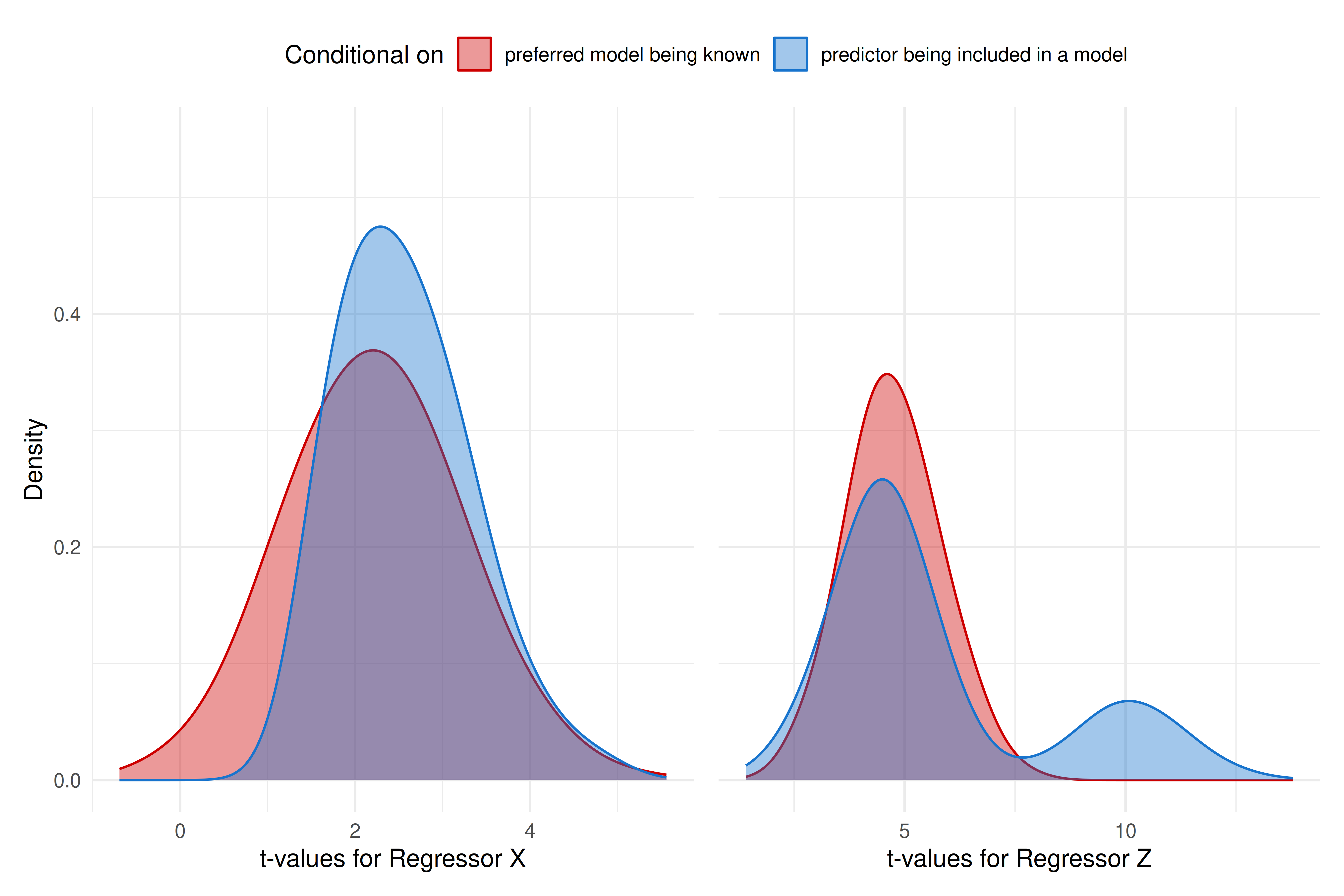
Note that Berk et al. (2010) uses the term preferred model instead of correct model. They do so because a model that excludes \(W\) can also be called correct the same as one like Equation 5, as long as \(\beta_1\) = 0 is allowed. To be consistent with the original text, we’ll use preferred to refer to the model with \(W\) excluded. This model is preferred because it generates the same conditional expectations for the response using up one less degree of freedom. The plots show the regression estimates t-values. “A distribution of t-values is more informative than a distribution of regression coefficients because it takes the regression coefficients and their standard errors into account” (Berk et al., 2010, p. 266).
reps =1000p <-3Sigma <-matrix(c(5,4,5,4,6,5,5,5,7), p, p)n =200betas <-c(3, 0, 1, 2)# values with model selectionrsq <-NULLcoefs <- cover <-matrix(NA, nrow = reps, ncol =3)colnames(coefs) <-c("w", "x", "z")colnames(cover) <-c("w", "x", "z")for (i inseq(reps)) { X <- MASS::mvrnorm(n = n, rep(0, 3) , Sigma) y <-as.numeric(cbind(1, X) %*% betas +rnorm(n, 0, 10)) Xy <-as.data.frame( cbind(X, y))colnames(Xy) <-c(c("w", "x", "z"), "y") fit <-lm(y ~ x + z, data = Xy) sel <-step(fit, k =2, trace =FALSE) s <-summary(sel) tvals <- s$coefficients[,3][-1] coefs[i, names(tvals)] <- tvals rsq[i] <- s$r.squared}# values without model selectionrsq_pref <-NULLcoefs_pref <- cover_pref <-matrix(NA, nrow = reps, ncol =3)colnames(coefs_pref) <-c("w", "x", "z")colnames(cover_pref) <-c("w", "x", "z")for (i inseq(reps)) { X <- MASS::mvrnorm(n = n, rep(0, 3) , Sigma) y <-as.numeric(cbind(1, X) %*% betas +rnorm(n, 0, 10)) Xy <-as.data.frame( cbind(X, y))colnames(Xy) <-c(c("w", "x", "z"), "y") fit <-lm(y ~ x + z, data = Xy) s <-summary(fit) tvals <- s$coefficients[,3][-1] coefs_pref[i, names(tvals)] <- tvals rsq_pref[i] <- s$r.squared}
xplot <- res_df |> dplyr::filter(sim %in%c("full", "x_included")) |>ggplot(aes(x, fill = sim, color = sim)) +geom_density(adjust =2, alpha =0.4) +theme_minimal(12) +theme(legend.position ="top") +scale_y_continuous(limits =c(0, 0.55)) +labs(x ="t-values for Regressor X", y ="Density") +scale_color_manual(name ="Conditional on",labels =c("preferred model being known", "predictor being included in a model"),values =c("red3", "dodgerblue3")) +scale_fill_manual(name ="Conditional on",labels =c("preferred model being known", "predictor being included in a model"),values =c("red3", "dodgerblue3"))zplot <- res_df |> dplyr::filter(sim %in%c("full", "z_included")) |>ggplot(aes(z, fill = sim, color = sim)) +geom_density(adjust =2, alpha =0.4) +theme_minimal(12) +theme(legend.position ="none",axis.title.y =element_blank(),axis.text.y =element_blank()) +scale_y_continuous(limits =c(0, 0.55)) +labs(x ="t-values for Regressor Z", y ="Density") +scale_color_manual(values =c("red3", "dodgerblue3")) +scale_fill_manual(values =c("red3", "dodgerblue3")) +guides(fill="none", color ="none")xplot + zplot +plot_layout(guides ='collect') &theme(legend.position='top')
Stepwise regression sampling distributions of the regression coefficient t-values for regressors X and Z. Red density plot is is conditional on the preferred model being known. The blue density plot is conditional on the regressor being included in a model
Code
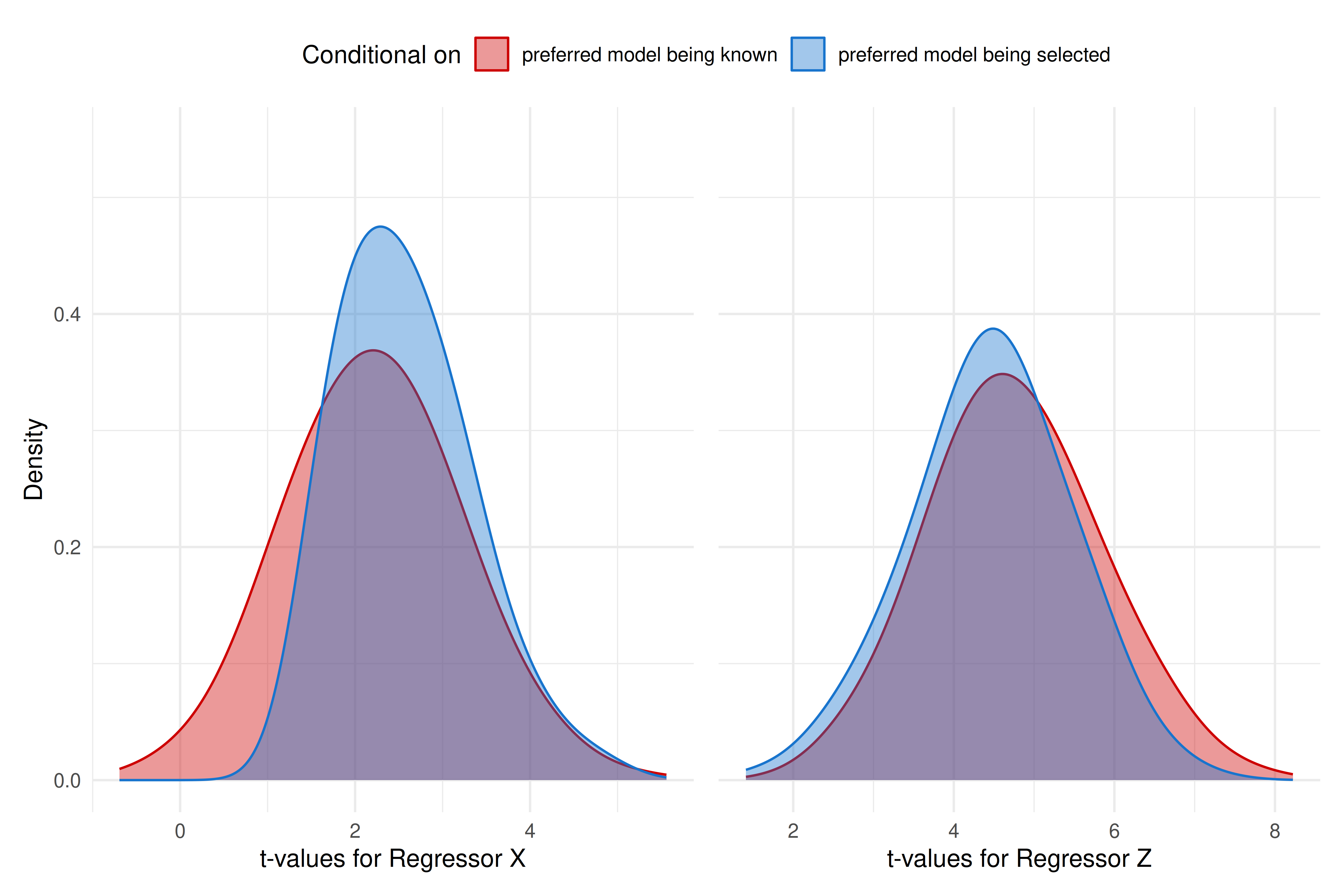
xpref_plot <- res_df |> dplyr::filter(sim %in%c("full", "pref")) |>ggplot(aes(x, fill = sim, color = sim)) +geom_density(adjust =2, alpha =0.4) +theme_minimal(12) +theme(legend.position ="top") +scale_y_continuous(limits =c(0, 0.55)) +labs(x ="t-values for Regressor X", y ="Density") +scale_color_manual(name ="Conditional on",labels =c("preferred model being known", "preferred model being selected"),values =c("red3", "dodgerblue3")) +scale_fill_manual(name ="Conditional on",labels =c("preferred model being known", "preferred model being selected"),values =c("red3", "dodgerblue3"))zpref_plot <- res_df |> dplyr::filter(sim %in%c("full", "pref")) |>ggplot(aes(z, fill = sim, color = sim)) +geom_density(adjust =2, alpha =0.4) +theme_minimal(12) +theme(legend.position ="none",axis.title.y =element_blank(),axis.text.y =element_blank()) +scale_y_continuous(limits =c(0, 0.55)) +scale_color_manual(values =c("red3", "dodgerblue3")) +scale_fill_manual(values =c("red3", "dodgerblue3")) +labs(x ="t-values for Regressor Z") +guides(fill="none", color ="none")xpref_plot + zpref_plot +plot_layout(guides ='collect') &theme(legend.position='top')
Stepwise regression sampling distributions of the regression coefficient t-values for regressors X and Z. Red density plot is is conditional on the preferred model being known. The blue density plot is conditional on the preferred model being selected
In both ?@fig-predinc and ?@fig-prefcond the red density plot represents the regression estimates t-values distribution when no model selection is performed. In ?@fig-predinc the blue density plot show the distributions when either \(X\) or \(Z\) are included in the model. For ?@fig-prefcond the blue distribution refers to distributions of either \(X\) or \(Z\)t-values when the preferred model is selected.
The contrast between red and blue curves are apparent. The difference that is the most striking are in t-values distributions post-model-selection for regressor \(Z\) when conditioned on the regressor being included in a model. This curve displays a bimodal distribution and highly biased mean and standard deviaton, as summarized below.
It is especially telling observing those plots that the assumed underlying distribution can be very different from what is obtained. Statistical inference performed in such scenarios would be misleading. ?@fig-prefcond confirms that conditioning on arriving at the preferred model does not guarantee trustable estimates.
Conclusion
Model selection methods are routine in research on the social and behavioral sciences, and commonly taught in applied statistics courses and textbooks. However, little is mentioned about the biased estimates obtained when such procedures are carried. With simulated data we have identified specific characteristics of the data generating model that can potentially increase the bias in estimates obtained through variable selection. Thus, we can conclude that post-model-selection sampling distribution can deviate greatly from the assumed underlying distribution, even when the best representative model of the data generation process has been selected.
Berk, R., Brown, L., Buja, A., Zhang, K., & Zhao, L. (2013). Valid post-selection inference. The Annals of Statistics, 41(2), 802–837. https://doi.org/10.1214/12-AOS1077
Berk, R., Brown, L., & Zhao, L. (2010). Statistical Inference After Model Selection. Journal of Quantitative Criminology, 26(2), 217–236. https://doi.org/10.1007/s10940-009-9077-7
Cohen, J., & Cohen, P. (1983). Applied Multiple Regression/Correlation Analysis for the Behavioral Sciences (2nd ed.).
Lukacs, P. M., Burnham, K. P., & Anderson, D. R. (2009). Model selection bias and Freedman’s paradox. Annals of the Institute of Statistical Mathematics, 62(1), 117. https://doi.org/10.1007/s10463-009-0234-4